Principle Componenets Analysis

I have tried to learn machine learning a few times. However, I never find the chance to implement any machine learning algorithm in my research. Here, I want to revisit the subject by reading Goodfellow’s book. I like simple things, because they help me understand the basic concept and gain intuition to the abstract math. Principle componenets analysis is such a simple thing, which I shall take some notes here to try to understand.

The problem – data compression

We want to compress a collection of points \( {x^{(1)}, …, x^{(m)}} \) in \(\mathbb{R}^n\) into code points \( {c^{(1)}, …, c^{(m)}} \) in \(\mathbb{R}^l\), where \( n>l \). We want an encode \( f(\mathbf{x})=\mathbf{c}\) and a decoder \( g(\mathbf{c}) \approx \mathbf{x}\).

A simple choice of the decoder is a matrix \( \mathbf{D} \) in \( \mathbb{R}^{n\times l}\), \( g(\mathbf{c}) = \mathbf{D}\mathbf{c}\). The goal is to find the best encoder and decoder, so that the distance between original points \(\mathbf{x}\) and the reconstructed points \(\mathbf{r}\) is minimized. Formally, we want to solve the following optimization:

where \( \mathbf{r} = g(f(\mathbf{x})) = \mathbf{D}f(\mathbf{x})\). To make the problem solvable, we need to figure out what is the encoder \(f(x)\). One way to do this is to make the distance between the reconstructed points closest to the original points, formally:

This is equivalent to

we can expand the square:

\(\mathbf{x}^\top\mathbf{x}\)is irrelevant since it does not contain \(\mathbf{c}\)we are optimizing. \(g(\mathbf{c})^\top \mathbf{x}\) and \(\mathbf{x}^\top g(\mathbf{c})\) are scalars, so they are equal. At this point, we can substitute the exact form of \(g(\mathbf{c})\), the objective function becomes

The 0-gradient point corresponds to a local minimum, which is the \(\mathbf{c}^*\) we are looking for.

The best encoder \(f(\mathbf{x})\) is found to be \(\mathbf{D}^\top\mathbf{x}\).

Next, we solve the optimization for \( \mathbf{D}^* \) to minimize the distance between original data \(\mathbf{x}\) and reconstruction \(\mathbf{r} = \mathbf{D}\mathbf{D}^\top\mathbf{x}\).

To simplify the derivation, we can look at a special case where \(l=1\), i.e. \(\mathbf{D}\) is \(\mathbb{R}^1\). We denote \(\mathbf{D}\) in this special case \(\mathbf{d}\), and rewrite the objective function

The summation can be written in a more compact form if we let \( \mathbf{X}_{i, :} = \mathbf{x}^{(i)\top} \), or

we can write the objective function as

stack all the \( \mathbf{x}^{(i)\top} \)

Here, the subscript \(_F\) denotes Frobenius norm, which measures the size of a matrix. This norm can be written in trace form:

\( \mathbf{X}^\top \mathbf{X} \) can be eigendecomposed into \( \mathbf{V}\mathbf{\Lambda}\mathbf{V}^\top \), where \( \mathbf{V} \) is the eigenvector matrix \( [ \mathbf{v}^{(1)} \dots \mathbf{v}^{(n)} ] \) and \( \mathbf{\Lambda} \) is the diagonal matrix of eigenvalues \( \text{diag}(\lambda_i) \). Substitute the eigendecomposition into the objective function, we get

Here \(\mathbf{d}^\top\mathbf{V}\) is a row vector. The result inside the trace is a scalar, and can be written as a summation of squares

If we ignore the eigenvalue coefficient, the summation \( \sum_i (\mathbf{d}^\top \mathbf{v}^{(i)})^2 \) is the sum of \( \mathbf{d} \) components in \( \mathbf{V} \) space, so it is 1. To maximize the objective function, the best strategy is to let the largest eigenvalue have the biggest weight, which leads to

that is, the best encoder and decoder set is the eigenvector that corresponds to the largest eigenvalue. This makes sense. The eigendecomposition maps the original data onto the eigenvector space. The largest eigenvalue denotes the longest component of the data set in this space.

More principle components can be shown to be other large eigenvectors by proof of induction. The key steps are:

1. when \(l = k\), assume

1. when \(l = k + 1\)

\(\mathbf{D’}=[\mathbf{D}, \mathbf{d}]\). Since \(\mathbf{D’}\) is orthogonal, we cannot have the same vectors. The best choice of \(\mathbf{d}\) is the eigenvector that corresponds to the largest eigenvalue, which is not already in \(\mathbf{D}\). Therefore,

It is also desired to have some examples of image compression. Let’s do a simple one.

import numpy as np

np.random.seed(0)
X = np.random.rand(100, 100) # random 2d array
XX = np.matmul(X.T, X) # X.T X
w, v = np.linalg.eig(XX) # eigendecomp

Then compute compression and reconstruction.

import matplotlib.pyplot as plt

for number_principle_components in [2, 50, 100]:
    D = v[:, :number_principle_components]
    C = D.T @ X
    R = D @ C

    fig, ax = plt.subplots(1, 2, figsize=(6, 3), dpi=100)
    ax[0].imshow(X)
    ax[1].imshow(R)

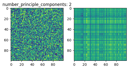
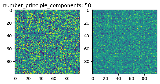
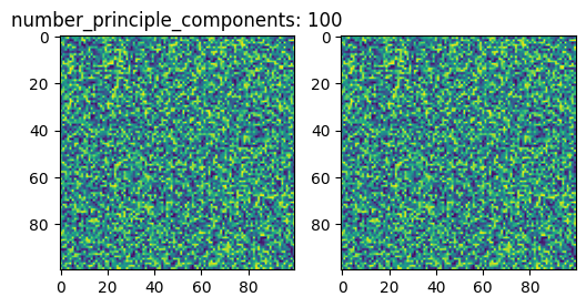
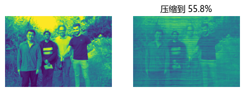
This is indeed a very simple compression algorithm, which does not recover good image quality.