White particles

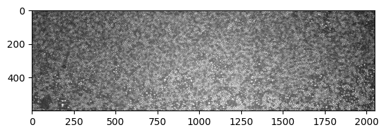
I received a new image from Qiaoge, with the majority of particles white. See below:

from skimage import io
import matplotlib.pyplot as plt
import numpy as np
from myimagelib.myImageLib import to8bit, matlab_style_gauss2D, bestcolor
from scipy.signal import convolve2d
from myimagelib.xcorr_funcs import normxcorr2, FastPeakFind
import pandas as pd
from skimage.feature import peak_local_max
from skimage import io, measure, draw
from bwtrack.bwtrack import *
from matplotlib.collections import PatchCollection

1 The old method

We can start by using the old find_white() function and see what is the problem.

def find_white(img, size=7, thres=None, std_thres=None, plot_hist=False):
    """
    Similar to find_black.
    """

    img = to8bit(img) # convert to 8-bit and saturate

    mh = mexican_hat(shape=(5,5), sigma=0.8) # 这里shape和上面同理，sigma需要自行尝试一下，1左右
    #plt.imshow(mh, cmap="gray")

    corr = normxcorr2(mh, img, "same")
    coordinates = peak_local_max(corr, min_distance=5)

    # apply min_dist criterion
    particles = pd.DataFrame({"x": coordinates.T[1], "y": coordinates.T[0]})
    # 加入corr map峰值，为后续去重合服务
    particles["peak"] = corr[particles.y, particles.x]
    particles = min_dist_criterion(particles, size)

    # 计算mask内的像素值的均值和标准差
    ## Create mask with feature regions as 1
    R = size / 2.
    mask = np.zeros(img.shape)
    for num, i in particles.iterrows():
        rr, cc = draw.disk((i.y, i.x), 0.8*R) # 0.8 to avoid overlap
        mask[rr, cc] = 1

    ## generate labeled image and construct regionprops
    label_img = measure.label(mask)
    regions = measure.regionprops_table(label_img, intensity_image=img, properties=("label", "centroid", "intensity_mean", "image_intensity")) # use raw image for computing properties
    table = pd.DataFrame(regions)
    table["stdev"] = table["image_intensity"].map(np.std)

    ## Arbitrary lower bound here, be careful!
    intensity_lb = (table["intensity_mean"].median() + table["intensity_mean"].mean()) / 4
    table = table.loc[table["intensity_mean"]>=intensity_lb]

    if thres is not None and std_thres is not None:
        table = table.loc[(table["intensity_mean"] <= thres)&(table["stdev"] <= std_thres)]
    elif thres is None and std_thres is None:
        print("Threshold value(s) are missing, all detected features are returned.")
    elif thres is not None and std_thres is None:
        print("Standard deviation threshold is not set, only apply mean intensity threshold")
        table = table.loc[table["intensity_mean"] <= thres]
    elif thres is None and std_thres is not None:
        print("Mean intensity threshold is not set, only apply standard deviation threshold")
        table = table.loc[table["stdev"] <= std_thres]

    if plot_hist == True:
        table.hist(column=["intensity_mean", "stdev"], bins=20)

    table = table.rename(columns={"centroid-0": "y", "centroid-1": "x"}).drop(columns=["image_intensity"])

    return table

img = io.imread("https://github.com/ZLoverty/bwtrack/raw/main/test_images/white.tif")
plt.imshow(img, cmap="gray")

<matplotlib.image.AxesImage at 0x203bd7dc670>

particles = find_white(img, size=7)

particles

	label	y	x	intensity_mean	stdev
0	1	5.0	7.0	115.142857	45.822719
1	2	5.0	26.0	101.476190	38.996697
2	3	5.0	240.0	84.761905	34.328996
3	4	5.0	315.0	137.666667	53.905755
4	5	5.0	359.0	62.095238	23.977790
...	...	...	...	...	...
9910	9911	594.0	1904.0	82.952381	34.009081
9911	9912	594.0	1912.0	81.142857	32.451416
9912	9913	594.0	1936.0	109.095238	44.550089
9913	9914	594.0	1943.0	102.857143	42.108431
9914	9915	594.0	1959.0	155.809524	61.843234

9822 rows × 5 columns

b_circ = [plt.Circle((xi, yi), radius=3.5, linewidth=1, fill=False, ec="magenta") for xi, yi in zip(particles.x, particles.y)]
b = PatchCollection(b_circ, match_original=True)
left, right, bottom, top = 1000, 1100, 300, 200
fig, ax = plt.subplots(dpi=100)
ax.imshow(img[top:bottom, left:right], cmap="gray", extent=(left, right, bottom, top))
ax.add_collection(b)

<matplotlib.collections.PatchCollection at 0x1d7cb121ee0>

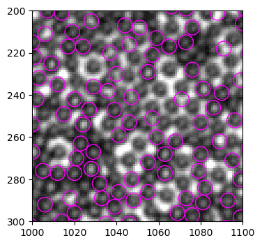
I have two general observations: - only part of the particles are identified - some bright “void” are identified as particles

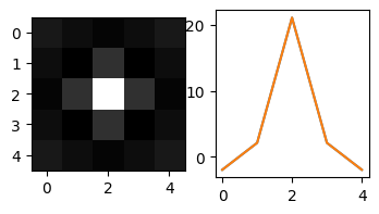
These problems suggests that the mask we use to detect white particles - the Mexican hat shape - does not capture the characteristics of white particles well, and therefore leads to false positives and missing particles. We briefly discussed this issue before. Basically, Mexican hat shape describes an intensity profile that has a high peak in the center and a low ring in the intermediate distance, and a medium value in the long distance:

We can take a few example particles and study precisely the intensity profiles. (probably we can use a polynomial profile to fit)

2 A closer look at the white particle pixel intensity profiles

In this section, we crop out several representative white particles and closely examine their intensity profiles, to determine the mask to use to detect them.

We choose particles from the four corners: 3115, 3197, 4155, 4014.

2.1 Particles that are found by find_white()

chosen = particles.query("label in [3115, 3197, 4155, 4014]")
size = 9

# show the cropped images
fig, ax = plt.subplots(nrows=1, ncols=4, figsize=(8, 2))
crop = {}
for i in range(4):
    item = chosen.iloc[i]
    x = int(item.x)
    y = int(item.y)

    crop[i] = img[y-size//2: y-size//2 + size, x - size//2: x - size//2 + size]
    ax[i].imshow(crop[i], cmap="gray")

# plot all the x, y center line profiles
fig, ax = plt.subplots(nrows=1, ncols=4, figsize=(8, 2), sharey=True)
for i in range(4):
    ax[i].plot(crop[i][3, :], label="x")
    ax[i].plot(crop[i][:, 3], label="y")
    if i == 0:
        ax[i].legend(frameon=False)

These four examples suggest that if we have a clear peak in the profile, find_white() can usually detect the particle.

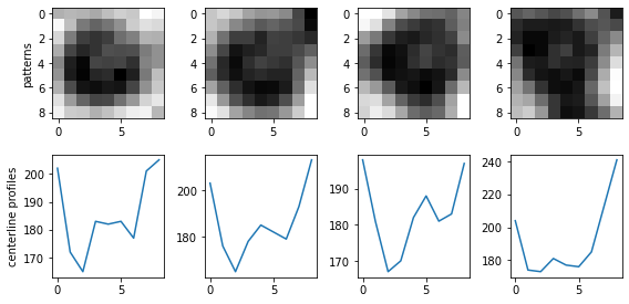
What’s more important is the particles that are not detected, because their common patterns give the direction to improve the tracking method. Let’s take a look.

2.2 Particles that are not detected

centers = ((1029, 226), (1065, 227), (1045, 271), (1072, 282))
fig, ax = plt.subplots(nrows=2, ncols=4, figsize=(8, 4))
i = 0
for x, y in centers:
    size = 9
    cropped = img[y-size//2: y-size//2+size, x-size//2: x-size//2+size]
    ax[0, i].imshow(cropped, cmap="gray")
    ax[1, i].plot(cropped[size//2, :])
    i += 1
ax[0, 0].set_ylabel("patterns")
ax[1, 0].set_ylabel("centerline profiles")
plt.tight_layout()

3 A better mask?

It turns out that Mexican hat is not the optimal mask for detecting white particles. Actually, in the old find_white function, the default Mexican hat mask mh is not even the same size as the paricles. The old default mask is:

mh = mexican_hat(shape=(5,5), sigma=0.8)
fig, ax = plt.subplots(nrows=1, ncols=2, figsize=(4, 2))
ax[0].imshow(mh, cmap="gray")
ax[1].plot(mh[2, :])
ax[1].plot(mh[:, 2])

[<matplotlib.lines.Line2D at 0x22d867aff70>]

3.1 Try different parameters of Mexican hat

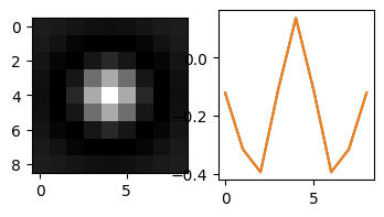
This is not really a Mexican hat, because the shape (5, 5) has truncated the profile before the tails rise again at long distances from the center peak. The mask (5,5) being smaller than the feature (D=7) could lead to the problem that many particles are not identified (because in the original image, a particle may not show up as a peak in a (5,5) region).

My intuition is, if I enlarge the size of the mask, while keeping the Mexican hat profile, I can get a better tracking. Let’s try the following mask.

mh = mexican_hat(shape=(9,9), sigma=1.5)
fig, ax = plt.subplots(nrows=1, ncols=2, figsize=(4, 2))
ax[0].imshow(mh, cmap="gray")
ax[1].plot(mh[2, :])
ax[1].plot(mh[:, 2])

[<matplotlib.lines.Line2D at 0x22d8246e430>]

def find_white(img, size=7, thres=None, std_thres=None, plot_hist=False):
    """
    Similar to find_black.
    """

    img = to8bit(img) # convert to 8-bit and saturate

    mh = mexican_hat(shape=(9,9), sigma=1.5) # 这里shape和上面同理，sigma需要自行尝试一下，1左右
    #plt.imshow(mh, cmap="gray")

    corr = normxcorr2(mh, img, "same")
    coordinates = peak_local_max(corr, min_distance=3)

    # apply min_dist criterion
    particles = pd.DataFrame({"x": coordinates.T[1], "y": coordinates.T[0]})
    # 加入corr map峰值，为后续去重合服务
    particles["peak"] = corr[particles.y, particles.x]
    # particles = min_dist_criterion(particles, size)

    # 计算mask内的像素值的均值和标准差
    ## Create mask with feature regions as 1
    R = size / 2.
    mask = np.zeros(img.shape)
    for num, i in particles.iterrows():
        rr, cc = draw.disk((i.y, i.x), 0.8*R) # 0.8 to avoid overlap
        mask[rr, cc] = 1

    ## generate labeled image and construct regionprops
    label_img = measure.label(mask)
    regions = measure.regionprops_table(label_img, intensity_image=img, properties=("label", "centroid", "intensity_mean", "image_intensity")) # use raw image for computing properties
    table = pd.DataFrame(regions)
    table["stdev"] = table["image_intensity"].map(np.std)

    ## Arbitrary lower bound here, be careful!
    intensity_lb = (table["intensity_mean"].median() + table["intensity_mean"].mean()) / 4
    table = table.loc[table["intensity_mean"]>=intensity_lb]

    if thres is not None and std_thres is not None:
        table = table.loc[(table["intensity_mean"] <= thres)&(table["stdev"] <= std_thres)]
    elif thres is None and std_thres is None:
        print("Threshold value(s) are missing, all detected features are returned.")
    elif thres is not None and std_thres is None:
        print("Standard deviation threshold is not set, only apply mean intensity threshold")
        table = table.loc[table["intensity_mean"] <= thres]
    elif thres is None and std_thres is not None:
        print("Mean intensity threshold is not set, only apply standard deviation threshold")
        table = table.loc[table["stdev"] <= std_thres]

    if plot_hist == True:
        table.hist(column=["intensity_mean", "stdev"], bins=20)

    table = table.rename(columns={"centroid-0": "y", "centroid-1": "x"}).drop(columns=["image_intensity"])

    return table

img = io.imread("large.tif")
particles = find_white(img, size=7)

Threshold value(s) are missing, all detected features are returned.

b_circ = [plt.Circle((xi, yi), radius=3, linewidth=1, fill=False, ec="magenta") for xi, yi in zip(particles.x, particles.y)]
b = PatchCollection(b_circ, match_original=True)
left, right, bottom, top = 1000, 1100, 300, 200
fig, ax = plt.subplots(dpi=100)
ax.imshow(img[top:bottom, left:right], cmap="gray", extent=(left, right, bottom, top))
ax.add_collection(b)
for num, i in particles.iterrows():
    ax.annotate(int(i["label"]), (i.x, i.y), xycoords="data", color="yellow", fontsize=6)

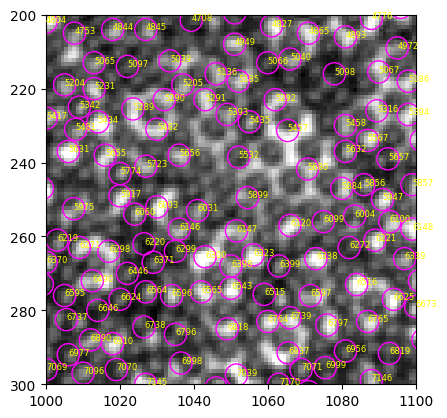
Even more bright “void” are mistakenly detected, suggesting that this modified MH is not a suitable mask.

3.2 Gaussian mask

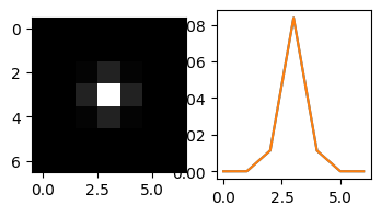
I have tried various shape and sigma for Mexican hat mask, but none of them work well for this image. Is there a better mask for this purpose? Gaussian mask might be the answer.

gs = matlab_style_gauss2D(shape=(7,7), sigma=0.5)
fig, ax = plt.subplots(nrows=1, ncols=2, figsize=(4, 2))
ax[0].imshow(gs, cmap="gray")
ax[1].plot(gs[2, :])
ax[1].plot(gs[:, 2])

[<matplotlib.lines.Line2D at 0x22dfec89220>]

def find_white(img, size=7, thres=None, std_thres=None, plot_hist=False):
    """
    Similar to find_black.
    """

    img = to8bit(img) # convert to 8-bit and saturate

    gs = matlab_style_gauss2D(shape=(7,7), sigma=3)
    #plt.imshow(mh, cmap="gray")

    corr = normxcorr2(gs, img, "same")
    coordinates = peak_local_max(corr, min_distance=3)

    # apply min_dist criterion
    particles = pd.DataFrame({"x": coordinates.T[1], "y": coordinates.T[0]})
    # 加入corr map峰值，为后续去重合服务
    particles["peak"] = corr[particles.y, particles.x]
    # particles = min_dist_criterion(particles, size)

    # 计算mask内的像素值的均值和标准差
    ## Create mask with feature regions as 1
    R = size / 2.
    mask = np.zeros(img.shape)
    for num, i in particles.iterrows():
        rr, cc = draw.disk((i.y, i.x), 0.8*R) # 0.8 to avoid overlap
        mask[rr, cc] = 1

    ## generate labeled image and construct regionprops
    label_img = measure.label(mask)
    regions = measure.regionprops_table(label_img, intensity_image=img, properties=("label", "centroid", "intensity_mean", "image_intensity")) # use raw image for computing properties
    table = pd.DataFrame(regions)
    table["stdev"] = table["image_intensity"].map(np.std)

    ## Arbitrary lower bound here, be careful!
    intensity_lb = (table["intensity_mean"].median() + table["intensity_mean"].mean()) / 4
    table = table.loc[table["intensity_mean"]>=intensity_lb]

    if thres is not None and std_thres is not None:
        table = table.loc[(table["intensity_mean"] <= thres)&(table["stdev"] <= std_thres)]
    elif thres is None and std_thres is None:
        print("Threshold value(s) are missing, all detected features are returned.")
    elif thres is not None and std_thres is None:
        print("Standard deviation threshold is not set, only apply mean intensity threshold")
        table = table.loc[table["intensity_mean"] <= thres]
    elif thres is None and std_thres is not None:
        print("Mean intensity threshold is not set, only apply standard deviation threshold")
        table = table.loc[table["stdev"] <= std_thres]

    if plot_hist == True:
        table.hist(column=["intensity_mean", "stdev"], bins=20)

    table = table.rename(columns={"centroid-0": "y", "centroid-1": "x"}).drop(columns=["image_intensity"])

    return table

img = io.imread("https://github.com/ZLoverty/bwtrack/raw/main/test_images/white.tif")
particles = find_white(img, size=7)

C:\Users\liuzy\Documents\Github\mylib\src\myimagelib\xcorr_funcs.py:42: RuntimeWarning: divide by zero encountered in divide
  out = out / np.sqrt(image * template)

Threshold value(s) are missing, all detected features are returned.

b_circ = [plt.Circle((xi, yi), radius=3, linewidth=1, fill=False, ec="magenta") for xi, yi in zip(particles.x, particles.y)]
b = PatchCollection(b_circ, match_original=True)
left, right, bottom, top = 1000, 1100, 300, 200
fig, ax = plt.subplots(dpi=100)
ax.imshow(img[top:bottom, left:right], cmap="gray", extent=(left, right, bottom, top))
ax.add_collection(b)

<matplotlib.collections.PatchCollection at 0x22dfc5be310>

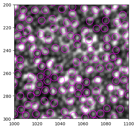
Compare with the original find_white result, we still don’t see much improvement:

3.3 Double well

It might help to use a mask based on the double well function:

\[f(x) = \frac{1}{4} x^4 - \frac{1}{2} x^2\]

the derivative of \(f(x)\) is

\[f'(x) = x^3 - x = x(x+1)(x-1)\]

and immediately see that \(x=-1, 0, 1\) are the local extrema in this function. Let’s plot \(f(x)\) below:

x = np.linspace(-2, 2)
y = x ** 4 / 4 - x ** 2 / 2
plt.plot(x, y)

[<matplotlib.lines.Line2D at 0x22d82abc190>]

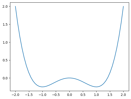
The results in section 2.2 show profiles similar to this double well pattern. Let’s construct the 2D version of this pattern:

\[f(r) = \frac{1}{4} r ^ 4 - \frac{1}{2} r ^ 2,\]

where \(r=\sqrt{x^2+y^2}\). This pattern always have minima at (-1, 1), therefore suitable for particles of size 2. To adapt it to other particle sizes, we can modify the prefactor of the \(r^2\) term. Say we are looking for particles of diameter \(d\), the mask should be

\[f(r) = \frac{1}{4} r ^ 4 - \frac{d^2}{8} r ^ 2.\]

In terms of \(x, y\):

\[f(x, y) = \frac{1}{4} (x^2 + y^2) ^ 2 - \frac{d^2}{8} (x^2 + y^2).\]

A preview of the mask is shown below, and \(d\) is set to 7.

size = 7
msize = size + 2
X, Y = np.mgrid[-msize/2: msize/2: msize*1j, -msize/2: msize/2: msize*1j]
mask = 1/4 * (X**2 + Y**2) ** 2 - size**2/8 * (X**2 + Y**2)
plt.imshow(mask, cmap="gray")

<matplotlib.image.AxesImage at 0x1d7cbb97fd0>

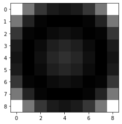
Now modify find_white() with the new double-well mask.

def find_white(img, size=7, thres=None, std_thres=None, plot_hist=False):
    """
    Similar to find_black.
    """

    img = to8bit(img) # convert to 8-bit and saturate

    # construct mask, only the following few lines are modified
    msize = size + 2 # set mask size to be larger than particle size by 2 pixels, this will make the double-well pattern more obvious
    X, Y = np.mgrid[-msize/2: msize/2: msize*1j, -msize/2: msize/2: msize*1j]
    dw = 1/4 * (X**2 + Y**2) ** 2 - size**2/8 * (X**2 + Y**2)

    corr = normxcorr2(dw, img, "same")
    coordinates = peak_local_max(corr, min_distance=3)

    # apply min_dist criterion
    particles = pd.DataFrame({"x": coordinates.T[1], "y": coordinates.T[0]})
    # 加入corr map峰值，为后续去重合服务
    particles["peak"] = corr[particles.y, particles.x]
    # particles = min_dist_criterion(particles, size)

    # 计算mask内的像素值的均值和标准差
    ## Create mask with feature regions as 1
    R = size / 2.
    mask = np.zeros(img.shape)
    for num, i in particles.iterrows():
        rr, cc = draw.disk((i.y, i.x), 0.8*R) # 0.8 to avoid overlap
        mask[rr, cc] = 1

    ## generate labeled image and construct regionprops
    label_img = measure.label(mask)
    regions = measure.regionprops_table(label_img, intensity_image=img, properties=("label", "centroid", "intensity_mean", "image_intensity")) # use raw image for computing properties
    table = pd.DataFrame(regions)
    table["stdev"] = table["image_intensity"].map(np.std)

    ## Arbitrary lower bound here, be careful!
    intensity_lb = (table["intensity_mean"].median() + table["intensity_mean"].mean()) / 4
    table = table.loc[table["intensity_mean"]>=intensity_lb]

    if thres is not None and std_thres is not None:
        table = table.loc[(table["intensity_mean"] <= thres)&(table["stdev"] <= std_thres)]
    elif thres is None and std_thres is None:
        print("Threshold value(s) are missing, all detected features are returned.")
    elif thres is not None and std_thres is None:
        print("Standard deviation threshold is not set, only apply mean intensity threshold")
        table = table.loc[table["intensity_mean"] <= thres]
    elif thres is None and std_thres is not None:
        print("Mean intensity threshold is not set, only apply standard deviation threshold")
        table = table.loc[table["stdev"] <= std_thres]

    if plot_hist == True:
        table.hist(column=["intensity_mean", "stdev"], bins=20)

    table = table.rename(columns={"centroid-0": "y", "centroid-1": "x"}).drop(columns=["image_intensity"])

    return table

img = io.imread("https://github.com/ZLoverty/bwtrack/raw/main/test_images/white.tif")
particles = find_white(img, size=7)

Threshold value(s) are missing, all detected features are returned.

b_circ = [plt.Circle((xi, yi), radius=3, linewidth=1, fill=False, ec="magenta") for xi, yi in zip(particles.x, particles.y)]
b = PatchCollection(b_circ, match_original=True)
left, right, bottom, top = 1000, 1100, 300, 200
fig, ax = plt.subplots(dpi=100)
ax.imshow(img[top:bottom, left:right], cmap="gray", extent=(left, right, bottom, top))
ax.add_collection(b)

<matplotlib.collections.PatchCollection at 0x1d7c7893ee0>

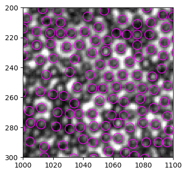
跟旧版find_white()的结果比较，找孤儿球的效果有显著提高，但同时在找非孤儿球时错误率提高。

4 Try find_black

Since we only have white particles in this image, they are actually the black ones compared to the background false positive. Let’s try find_black, see if it works better.

img = io.imread("https://github.com/ZLoverty/bwtrack/raw/main/test_images/white.tif")
particles = find_black(img, size=7)

Threshold value(s) are missing, all detected features are returned.

b_circ = [plt.Circle((xi, yi), radius=3, linewidth=1, fill=False, ec="magenta") for xi, yi in zip(particles.x, particles.y)]
b = PatchCollection(b_circ, match_original=True)
left, right, bottom, top = 1000, 1100, 300, 200
fig, ax = plt.subplots(dpi=100)
ax.imshow(img[top:bottom, left:right], cmap="gray", extent=(left, right, bottom, top))
ax.add_collection(b)

<matplotlib.collections.PatchCollection at 0x22dfc096610>

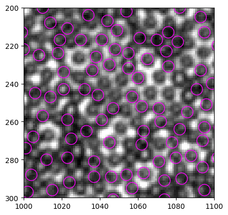
Compare with the results of find_white:

It start to be interesting! Both methods detects part of the particles, but neither out performs the other.

There are several difficult things in this tracking task:

• the image resolution is low, only a few tens of pixels can be used to determine if a pattern is a particle or not

• the aggregation significantly changes how the particles appear in the images, they are darker in aggregates, in particular the edges.

• when particles are dense, the void spaces also look like particles because they also have bright centers and dark edges (which are actually particle edges, but of other real particles). But I think these false positives can be easily removed by thresholding the mean intensity.

But, find black still does not work as well as the double-well mask.

5 Add more optional args to find_white()

• mask_size

• mask_pattern

def find_white(img, size=7, mask_size=None, mask_pattern="dw", thres=None, std_thres=None, plot_hist=False):
    """
    Find "white" particles in Qiaoge's images of particles at water-oil interface.

    :param img: input image
    :param size: particle size to look for (px)
    :param mask_size: mask (template) image size (px). By default, ``mask_size`` is set to ``size+2``. Making mask slightly larger can help making the correlation map sharper, sometimes.
    :param mask_pattern: choose from "mh", "gs" and "dw", which stands for mexican hat, gaussian and double well, respectively.
    :param thres: mean intensity threshold, meant to discern white particles from black particles.
    :param std_thres: standard deviation threshold, meant to discern white particles from black particles.
    :plot_hist: if True, plot mean intensity and standard deviation histogram. This can help you to determine good threshold values. Set to False when doing batch tracking (default).
    :return particles: a list of particle coordinates detected.
    """
    if mask_size == None:
        mask_size = size + 2 # set default mask_size value

    # construct mask
    if mask_pattern == "dw":
        X, Y = np.mgrid[-mask_size/2: mask_size/2: mask_size*1j, -mask_size/2: mask_size/2: mask_size*1j]
        tpl = 1/4 * (X**2 + Y**2) ** 2 - size**2/8 * (X**2 + Y**2)
    elif mask_pattern == "mh":
        tpl = mexican_hat(shape=(mask_size, mask_size), sigma=0.8) # sigma here is still arbitrary, I don't know how to set a more heuristic value yet
    elif mask_pattern == "gs":
        tpl =matlab_style_gauss2D(shape=(mask_size, mask_size), sigma=mask_size/3)

    img = to8bit(img) # convert to 8-bit and saturate

    corr = normxcorr2(tpl, img, "same")
    coordinates = peak_local_max(corr, min_distance=5)

    # apply min_dist criterion
    particles = pd.DataFrame({"x": coordinates.T[1], "y": coordinates.T[0]})
    # 加入corr map峰值，为后续去重合服务
    particles["peak"] = corr[particles.y, particles.x]
    # particles = min_dist_criterion(particles, size)

    # 计算mask内的像素值的均值和标准差
    ## Create mask with feature regions as 1
    R = size / 2.
    mask = np.zeros(img.shape)
    for num, i in particles.iterrows():
        rr, cc = draw.disk((i.y, i.x), 0.8*R) # 0.8 to avoid overlap
        mask[rr, cc] = 1

    ## generate labeled image and construct regionprops
    label_img = measure.label(mask)
    regions = measure.regionprops_table(label_img, intensity_image=img, properties=("label", "centroid", "intensity_mean", "image_intensity")) # use raw image for computing properties
    table = pd.DataFrame(regions)
    table["stdev"] = table["image_intensity"].map(np.std)

    ## Arbitrary lower bound here, be careful!
    intensity_lb = (table["intensity_mean"].median() + table["intensity_mean"].mean()) / 4
    table = table.loc[table["intensity_mean"]>=intensity_lb]

    if thres is not None and std_thres is not None:
        table = table.loc[(table["intensity_mean"] <= thres)&(table["stdev"] <= std_thres)]
    elif thres is None and std_thres is None:
        print("Threshold value(s) are missing, all detected features are returned.")
    elif thres is not None and std_thres is None:
        print("Standard deviation threshold is not set, only apply mean intensity threshold")
        table = table.loc[table["intensity_mean"] <= thres]
    elif thres is None and std_thres is not None:
        print("Mean intensity threshold is not set, only apply standard deviation threshold")
        table = table.loc[table["stdev"] <= std_thres]

    if plot_hist == True:
        table.hist(column=["intensity_mean", "stdev"], bins=20)

    table = table.rename(columns={"centroid-0": "y", "centroid-1": "x"}).drop(columns=["image_intensity"])

    return table

img = io.imread("https://github.com/ZLoverty/bwtrack/raw/main/test_images/white.tif")
# reproduce old version behavior (mh mask, size=7, mask_size=5)
particles_old = find_white(img, size=7, mask_size=5, mask_pattern="mh")
# new double-well template (dw mask, size=7, mask_size=9)
particles = find_white(img, size=7, mask_size=9, mask_pattern="dw")

fig, ax = plt.subplots(ncols=2, figsize=(10, 5))
left, right, bottom, top = 1000, 1100, 300, 200 # set ROI

b_circ = [plt.Circle((xi, yi), radius=3, linewidth=1, fill=False, ec="magenta") for xi, yi in zip(particles_old.x, particles_old.y)]
b = PatchCollection(b_circ, match_original=True)
ax[0].imshow(img[top:bottom, left:right], cmap="gray", extent=(left, right, bottom, top))
ax[0].add_collection(b)
ax[0].set_title("mexican hat")

b_circ = [plt.Circle((xi, yi), radius=3, linewidth=1, fill=False, ec="magenta") for xi, yi in zip(particles.x, particles.y)]
b = PatchCollection(b_circ, match_original=True)
ax[1].imshow(img[top:bottom, left:right], cmap="gray", extent=(left, right, bottom, top))
ax[1].add_collection(b)
ax[1].set_title("double well")

C:\Users\liuzy\Documents\Github\mylib\src\myimagelib\xcorr_funcs.py:42: RuntimeWarning: divide by zero encountered in true_divide
  out = out / np.sqrt(image * template)

Threshold value(s) are missing, all detected features are returned.
Threshold value(s) are missing, all detected features are returned.

Text(0.5, 1.0, 'double well')

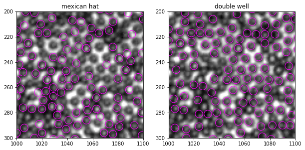
With more optional args, we can experiment more the effect of mask_pattern and mask_size. The current arg set (size=7, mask_size=9, mask_pattern="dw") already gives good improvement.

6 Minimal example

from bwtrack.bwtrack import *
from skimage import io

img = io.imread("https://github.com/ZLoverty/bwtrack/raw/main/test_images/white.tif")
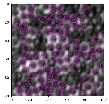
particles = find_white(img)
fig, ax = show_result(img, particles, size=7)

Threshold value(s) are missing, all detected features are returned.

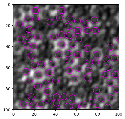
size = 6
particles = find_white(img, size=size)
fig, ax = show_result(img, particles, size=size)

Threshold value(s) are missing, all detected features are returned.

img = io.imread("https://github.com/ZLoverty/bwtrack/raw/main/test_images/white.tif)
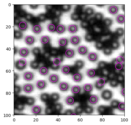
particles = find_white(img, size=6, mask_size=7)
fig, ax = show_result(img, particles, size=6)

C:\Users\liuzy\Documents\Github\mylib\src\myimagelib\xcorr_funcs.py:42: RuntimeWarning: divide by zero encountered in divide
  out = out / np.sqrt(image * template)
C:\Users\liuzy\Documents\Github\mylib\src\myimagelib\xcorr_funcs.py:42: RuntimeWarning: invalid value encountered in divide
  out = out / np.sqrt(image * template)

Threshold value(s) are missing, all detected features are returned.

plt.imshow(img, cmap="gray")

<matplotlib.image.AxesImage at 0x2a7cf8fe6d0>